There are many situations where we want to display a large quantity and diversity of data, and at the same time show details — or at least show that details exist and are easily accessible. Isn't this contradictory: both quantity and details? Nonlinear projections can help, or at least make it fun to explore.
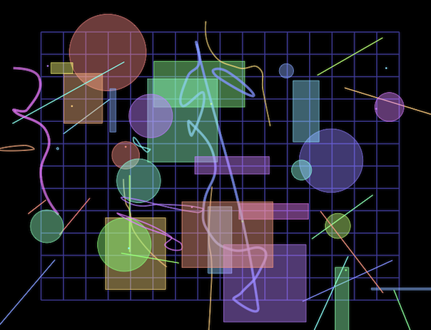
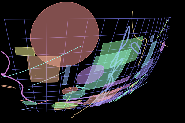
The screen shots at the right show where we're going. The upper one is a flat view of some shapes and a background grid. The lower shows the result of a click on the red circle at the upper left: the image has zoomed to bring the clicked object into closer view, but at the same time has slewed and distorted so that we can still see our entire object universe around the edges. The farther away from where we clicked, the more distorted the shapes are. It is exactly as if we had a fisheye lens over the image. See for yourself now, then come back for an explanation of what's going on.
The demo uses the usual primitive shapes — points, lines, rectangles, circles — to show how the fisheye projection works. The circle implementation is general, so ellipses can easily be included by setting their width different from their height. But the interesting shapes are the odd squiggles and loops: those are interpolating spline curves which you can learn about (and find the code to generate and display). They're included here to show that their implementation is general, that their geometry can be smoothly distorted the same as the more basic shapes.
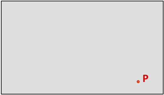
We begin with a set of data in two-dimensional graphic form, perhaps any of the methods you'll see elsewhere on this site: a treemap, dendrogram, network diagram, anything. It will be more useful if the data are naturally layered, so that when the user zooms in, more details can be gently revealed. In the sketch, we consider simply how to map point P, which can be anywhere in the gray rectangle which surrounds all of the data.
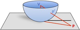
Next we drop a fisheye lens on the plane. We have control over the radius of the lens and where we place it; these are important parameters which affect the final image. Point p' is the projection of P onto the surface of the lens, as seen from a viewer at the center of the lens V. The lens should have zero slope where it contacts the plane, so that objects directly under it are rendered smoothly. The lens should be a monotonic curve without creases or folds. Also the height of the viewpoint V defines the rim of the lens: nothing above the rim matters, since the rim projects to infinity. In other words, no matter how far away point P is, if it's in the gray plane of the data, it's guaranteed to have a unique projection p' under the rim. This is the geometry that lets us depict huge spaces in a way that's "actual size" right under the lens, and squeezed toward the rim. Note that the lens does not have to be a hemisphere, it can be any shape that meets the above criteria, and the point V doesn't need to be at its center. It's just that spheres and parabolas are useful because the length of an arc on their surfaces is easily calculated.
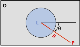
The next sketch is a top view of the plane and the lens. Our data have a coordinate origin, which can be anywhere but in computer screen convention is at the top left, marked O. Now we see the point L where the lens touches the plane; it's directly under V. Point P is distance R from L, and this line has angle θ from the x-axis of the data coordinate system.
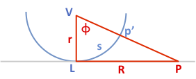
Switching to a side view sliced through the blue lens, we have the diagram we need to find the above-the-plane information. The lens is now just a blue semicircle (or parabola, or whatever shape we chose). The projection from P up to V passes through the lens at p', forming a right triangle with angle φ at V. That's about it: we know the coordinates of the points and the lengths r and R. If the lens is a hemisphere, the arc length s is just rφ.
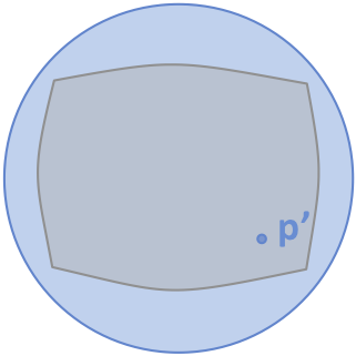
To display the distorted view that's been projected onto the surface of the lens, we just smoothly flatten that surface down onto the plane (this is topology, where everything's made of rubber sheets and perfectly flexible). This is very easy: pick a point as the center of the new image, drop angle θ from the horizontal, go out distance s, and draw projected point p'. Because s can't exceed πr/2 (1/4 circumference = 2πr/4 = πr/2), any point closer than infinity maps smoothly onto the new image. Depending on the chosen radius of the lens and any additional planar magnification added, the edges of the original rectangular data space will appear pillow-shaped.
This trigonometry is so simple that it's easy to derive the return function: given the properties of the fisheye lens (its position and radius), and where the user clicked the mouse (on point p', which is what we show on the screen), we can readily back-calculate to find the coordinates of the point P in data-space, and with that information, we can do useful things like highlight and reveal more detail based on the underlying data. In the demo, clicking creates a little red and white target, which notably is in the data space, not just the frame of the screen.
How the animation works: It is absolutely worth the trouble to create a high-level abstraction (like the high school geometry above) for such nonlinear mappings when it comes time to animate between views. "Curvature" in the demo is just a unit-free abstraction of the radius of the fisheye lens, and "magnification" is just a linear zoom applied after the nonlinear stuff. Where you click becomes (in data space) the next spot "where the lens touches the paper." All that's needed to animate is linear interpolation of these four parameters between the old and new views. The drawing routine is based on the abstract data model, so just redrawing every 30 milliseconds with the interpolated parameters does the trick.